Notes to readers: This paper provided a basic user's guide for ACS staff members to Lynn Conway's MPM Architectural/RTL Timing Simulator for the ACS-1 MPM  (Main Processor Module).. The paper is of historical interest because it reveals the scope of the ACS-1 simulation capability, and because it also reveals details of the ACS-1's out-of-order multiple instruction issuance (3 out of 8) dynamic instruction scheduling subsystem running in action,via a detailed simulation input/output example below.

 

This page was created by scanning and OCR'ing the original IBM-ACS internal paper. Page numbers correspond to the original. See the following link for a scanned PDF of the original paper. (PDF)  

 

This paper has been officially declassified by IBM, and Lynn Conway has been granted a worldwide license to distribute it for historical and academic purposes. For background and context on this paper, refer to Lynn Conway's ACS-Archive Front-Matter.

 

 

IBM CONFIDENTIAL

 

August 25, 1967
Advanced Computing Systems
Menlo Park

 

 

MPM Timing Simulation
ACS AP #67-115

 

 

Reference:

1. ACS AP #66-022, ACS Simulation Technique
2. ACS-1 MPM Instruction Manual
3. ACS AP #67-068, MPM-Instruction Sequencing

 

To: File

 

[signature]

 

L. Conway

LC:slb

 

 

 

IBM CONFIDENTIAL

 

CONTENTS

 

0-1 Introduction

1-1 The Unroller

2-1 The Timing Simulator

3-1 Current Job Running Procedures

4-1 Table of Implemented Instructions

5-1 Planned Modifications

 

 

0-1
IBM CONFIDENTIAL

 

 

INTRODUCTION

 

This memo describes the programs which perform MPM timing simulation, It is primarily a "users manual" for these programs.

 

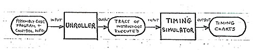
Two programs, the Unroller and the Timing Simulator, are ran consecutively in order to time the MPM's execution of a user's input program.

 

The Unroller program accepts an ACS assembly language program and control information concerning branch and skip execution, and it unrolls" the program to produce a trace of the instructions executed by the MPM when running the program. The trace is the sequence of instructions along with their addresses, register fields, and certain other information.

 

The Timing Simulator then operates on the trace of instructions executed by the MPM and produces timing charts indicating the timing of the activities initiated by these instructions in the various hardware components of the MPM.

 

The following diagram illustrates the functions and relationships of these two programs.

 

 

 

In the following sections of the memo, these programs are separately described with examples given illustrating preparation of input and interpretation of output.

 

The job running procedures for using the programs is described, and the MPM ops currently implemented in the Timing Simulator are listed.

 

Since the programs are currently undergoing changes, the current and planned changes are described to assist users in their planning.

 

Criticisms and suggestions from potential users are welcome and will be helpful in making the Timing Simulator useful to ACS.

 

 

1-1

IBM CONFIDENTIAL

 

 

THE UNROLLER PROGRAM (Prog. by J. Novicki, CSC)

 

The Unroller program produces the input trace to the Timing Simulator from an ACS assembly-code program plus control information.

 

In the past an Execution Simulator, which performed a detailed simulation of the execution of an input program, was used to generate the instruction trace. It was found to be inconvenient to use an execution simulator for this purpose because that requires the accurate programming of all the tests and computations which determine the desired path of execution through the program. It often proved to be difficult and time consuming to write a correctly executing program even though the path to be followed was easily described.

 

The Unroller program was written to solve this problem. Given an ACS assembly language program, explicit indicators are placed on the branch and skip instructions of the program to determine the path of instruction execution. For example a branch op might be followed by (3 BEGIN, *) to indicate that the first three times the branch is executed it is successful with the branch being to the instruction labelled BEGIN, and the fourth time the branch is executed it is unsuccessful.

 

This program and control information is processed by the Unroller to yield the trace of instructions executed, which may then be used as input to the Timing Simulator.

 

Input Language, Card Input Format

 

Input cards may contain a label, an op, code and operands. The Branch and Skip instructions may contain additional control information. A free' form format is used with no fixed starting columns for each of these fields but with certain delimiter restrictions. An asterisk In column I indicates a comment card.

 

Label: A label can be up to 8 characters maximum and must start with one of the characters A through Z or $. A label can contain no imbeded blanks and must be terminated by a delimiting colon.

 

Op Code: An op, code can be up to 6 characters long with no embedded blanks. It may be immediately followed by an asterisk to indicate the Skip flag. At least one blank column must be between the op code and its operand fields.

 

 

1-2
IBM CONFIDENTIAL

 

 

Operands: The operand fields can contain information for the i, j, k, and h fields of the instruction. Two fields must be separated by a comma and a missing field will be indicated by two consecutive commas. The first blank column terminates the operand fields. The i, j, and k fields may be one of the following formats:

 

(i) Ldd
(ii) dd

 

where "L" is the letter A for Arithmetic Register or the letter X for Index Register or the letter C for Condition Register or the letter S for Special Register. '"dd" is a decimal number from 00 to 31 (leading 0 may be omitted). The h field may contain a symbolic label or a decimal number (up to 5 digits).

 

Branch Parameters: A string of control parameters may be listed after a branch instruction to determine the path of instruction sequencing. The parameters indicate if the branch is successful or unsuccessful for each time it is executed. The branch parameter information must begin with a left parenthesis and end with a right parenthesis and contains no imbedded blanks. Two parameters in the list must be separated by a comma. The parameter format is:

 

(i) dL for a successful branch
(ii) d* for an unsuccessful branch

 

where d is an optional digit indicating the number of times the branch is successful or unsuccessful, L is the symbolic label of the instruction branched to, and * is an indicator for an unsuccessful branch. For example, if we have the instruction

 

BEQ C1, C2, X4 (3ABC, *, XY)

 

the program would be expanded to reflect the branch execution as follows:

 

(i) first three executions of branch are successful and branch is to instruction labelled ABC

(ii) fourth execution of branch is unsuccessful
(iii) fifth execution of branch is successful - to XY

 

Skip Parameters: A string of control parameters may be listed after a skip instruction to determine the effect of that instruction on the sequence of skip states. The parameters indicate whether the skip is taken or not, taken each time it is executed. The parameter string

 

 

1-3
IBM CONFIDENTIAL

 

 

has the same format as the branch parameter string with any dummy label serving to indicate that the skip is taken, an * indicating the skip is not taken. For example, if we have

 

SKOR C1, C2 (2*, LABEL, *)

 

the Unroller would set the skip state in the trace to reflect the execution of the skip as follows:

 

(i)first two times skip is executed it is not taken

(ii) third time skip is executed it is taken
(iii) fourth time skip is executed it is not taken

 

 

Output of Unroller

 

Corresponding to the sequence of execution of the instructions of the input program the Unroller produces the standard input trace for the Timing Simulator: a card deck which is described in detail in Section 2. One card is produced for each instruction executed. The card contains the op, i, j, k, h fields, branch and skip states, instruction and data reference addresses and certain other fields.

 

The Unroller also lists the input program and output trace. Certain diagnostic messages may be listed:

 

(i) Too many input cards (300 maximum)
(ii) Operand Field error
(iii) Error on following card (i. e. label information error)
(iv) Op code on next card not implemented

 

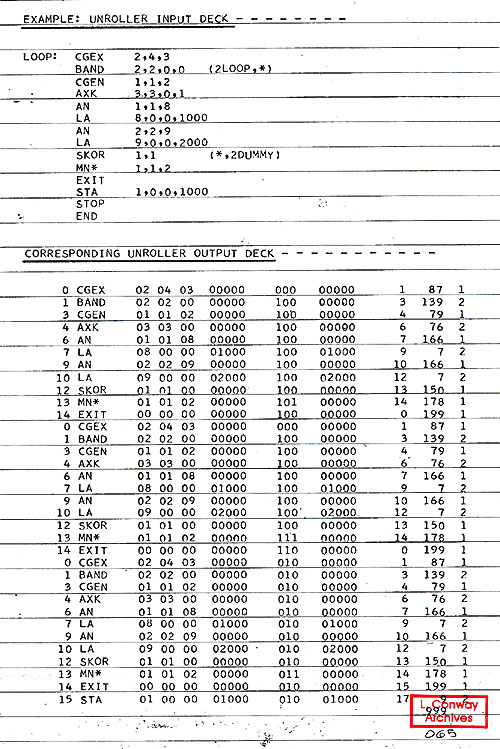
Example: On the following page are the listings of a simple input program deck and the trace deck produced by the Unroller from that input deck. Note that the branch parameter list specifies branch successful two times then branch unsuccessful. Thus we make 3 passes through the loop. The branch and skip states in the trace (see trace format Section 2) reflect the branch and skip execution. Note: the OP "STOP" terminates unrolling, and the pseudo op "END" marks the end of the unroller input deck.

 

 

1-4

 

 

2-1
IBM CONFIDENTIAL

 

 

THE TIMING SIMULATOR (Prog. by L. Conway, J. F. Parsons)

 

For the purpose of MPM hardware or program evaluation we may need detailed timing of the execution of a program by the MPM. The MPM is sufficiently complex that hand-timing of all but trivial programs is a very tedious process. The Timing Simulator is a program written to perform this timing by simulating in complete detail the hardware controls of the MPM.

 

The Timing Simulator is written in FORTRAN IV (H) and runs on a S/360 under OS, requiring an H level machine. The simulation technique is similar to SIMSCRIPT but uses simpler utility routines which are written in FORTRAN. Reference I provides a complete description of the simulation technique.

 

The level of hardware modelling performed by the Timer is best described as being an "architectural" level. Individual hardware triggers are included when they serve an individual control function, but buses, registers, etc., are modelled as logical entities rather than simulated to the bit level. Thus the timer does not model the detailed engineering implementation of the MPM. It does model all control algorithms in all sections of the MPM, to accurately simulate the timing of instruction execution by the MPM.

 

The Timer currently operates on a MOD 75 at a rate of approximately 10 simulated machine cycles per second. Typical programs are thus simulated at a rate of 20 inst./sec.

 

A detailed description of either the Timing Simulator program or the MPM model simulated is beyond the scope of this memo. Users may assume that the program reflects the latest specification of the MPM. This model is documented at an architectural level in Reference 3 and other similar references soon to be issued. Those who are familiar with the hardware design of the MPM and have specific questions about the details of the simulation model should contact the author.

 

The remainder of this section on the Timer is concerned with the practical problems of preparing input and interpreting the output timing charts.

 

The input to the timer is a "trace" of the instructions actually executed by the program to be timed. The trace consists of the sequence of instructions executed along with certain control information. This input is prepared by running an ACS assembly code program through the Unroller program (see Section 1).

 

 

2-2
IBM CONFIDENTIAL

 

 

Certain job controlling cards including a specification of the hardware parameters for the run are added to the trace deck to form the input deck.

 

The output of the Timer is a series of timing charts which illustrate the activities initiated by the instructions of the input program trace in the various hardware components of the MPM as a function of time.

 

A detailed description of the input and output formats and output interpretation is given on the following pages. Examples are given which follow the paths of individual instructions through the various sections of the MPM as a function of time.

 

 

Timing Simulator Input Preparation

 

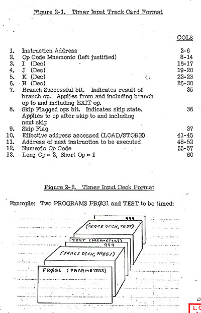
Input Trace Cards: The Unroller program is used to produce the input trace card decks for the Timing Simulator. An ACS assembly code program is run on the Unroller and a trace deck is produced as output. Refer to Section 1 for information on this program. The trace deck produced by the Unroller is an instruction by instruction record of those instructions actually executed by the program to be timed. Each instruction of the trace is present on a separate card. The format of these cards is specified in Fig. 2-1.

 

Timer Input Deck Format: Each program to be timed is formed into one deck beginning with a machine parameter card, followed by the trace cards for the program, and ending with a card containing 999 in cols 55, 56, 57 (a "STOP" card). A number of such input decks may be stacked and timed during one execution of the Timer. An example of this stacked job deck structure is illustrated in Fig. 2- 2.

 

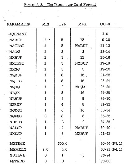
Parameter Card: The first card of each input program deck is a parameter card which specifies certain MPM hardware parameter values and certain parameters for the running of the job (maximum simulated time, etc.). These parameters are the following:

 

JOBNAME: Up to six characters identifying program

 

NABUF, NATEST, NAGO: The number of A Buffers, the number tested each cycle for OP issuance, the maximum number of OP which may be issued for execution each cycle from the A Buffers (A Contending Stack).

 

NXBUF, NXTEST, NXGO: Similarly for X unit Contending Stack.

 

 

2-3
IBM CONFIDENTIAL

 

 

NQBUF, NQTEST, NQGO: Similarly for Data Memory Queue.

 

NBOX: Number of memory boms.

 

NBBUF, NSBUF: Number of Exit History Table positions, number of Skip Table positions.

 

NODOT: Number of DO Table positions.

 

NOPSC: Number of PSC registers.

 

NDBUS: Number of Dispatcher Buses.

 

NADSP: Maximum number of OPS which maybe dispatched to the A Buffer per cycle.

 

NXDSP: Similarly for X dispatching.

 

MXTIME: Run control parameter. Maximum simulated time allowed for run (in machine cycles). Run terminated if this time is exceeded.

 

MEMDLY: Memory Delay Time. See example of arithmetic load G7 on page 2-13 for exact definition.

 

OUTLVL: One of four output levels maybe chosen. Level 0 is most detailed, Level 3 is least detailed (and fastest cunning). Level 1 is normally used and is level shown in the examples at the end of this section.

 

FSTADD: Starting address of the input program.

 

Fig. 2-3 specifies the format of the parameter card. Minimum, typical,
and maximum values of the parameters are given. The TYP values
represent the "most likely" values of the hardware parameters.

 

There are other machine parameters not controlled by the parameter card which may be easily varied by changing certain initialization tables in the Timer. An example of this is the busing and facility characteristics in the A and X execution units; These structures are listed in the output for each run (see output portion of this section). If changes in these machine parameters are desired for a particular timing study, contact the author.

 

 

2-4

 

 

2-5

 

 

2-6
IBM CONFIDENTIAL

 

 

Timing Simulator Output Interpretation

 

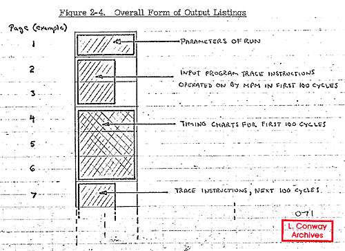
For each input job, a deck headed by a parameter card and terminated by a 999 card, an output listing is produced of the following form:

 

(i) The first page lists the job name and all parameters of the run including the busing and facility structure.

 

(ii) This is followed by a listing of those input trace instructions operated upon by the MPM during the first 100 simulated cycles of time.

 

(iii) This is followed by a listing of timing charts indicating the activities initiated by those instructions of (ii) during the first 100 simulated cycles.

 

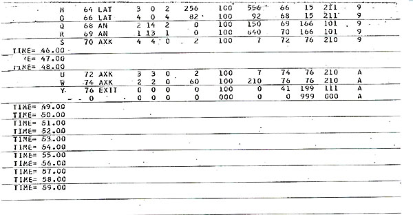
(iv) Items (ii) and (iii) are repeated for successive 100 cycle periods till the run stops or is terminated by MXTIME.

 

 

 

2-7
IBM CONFIDENTIAL

 

 

We will now examine the general characteristics of these three components of the output. A sample output listing is included at the end of the section for reference while studying these general descriptions.

 

Some specific examples will then be developed which illustrate the progression of instruction activity through the different sections of the MPM. These examples are referenced by markers on the sample output listings.

 

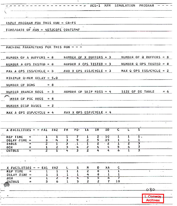
Parameters of Run: This page lists the job name, date and time of run, and the MPM hardware parameters for the run. Many of these parameters are those specified on the input parameter card, described earlier in this section. The A and X unit busing and facility structures are printed for reference in a table with the following entries:

 

1. The abbreviated name of the facility (FA1 = floating adder 1).

2. The Rep Time of the facility - the number of cycles an operation keeps the facility busy.

3. The Delay Time of the facility - the number of cycles the facility requires to perform operation.

4. INBUS - the numbers assigned indicate which facilities share a common inbus.

5. BOX - the numbers assigned show which facilities share circuitry and cannot be simultaneously busy.

6. OUTBUS - the numbers indicate which facilities share a common outbus.

 

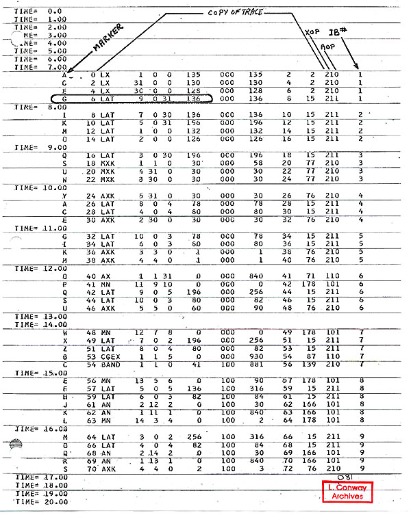
Input Program Trace: For each block of 100 cycles of simulated time the Timer prints the instructions of the input trace which have been operated upon by the MPM during that time. This is used to reference the timing charts for that period of time. The input program trace printed is a copy of the input cards with five fields added:

 

(i) Time markers are placed indicating the time (approx.) that the instruction entered an IB.

 

(ii) A letter is assigned to each instruction by decoding the instruction address MOD 26. This letter is then used as the marker for that instruction in the timing charts.

 

 

2-8
IBM CONFIDENTIAL

 

 

(iii), (iv) Bits are set indicating whether the op is to be dispatched to the A unit, X unit or both.

 

(v) The number of the IB into which the instruction was fetched.. This along with (i) will locate the instruction marker's first appearance on the timing charts (in a dispatch register).

 

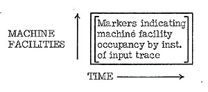
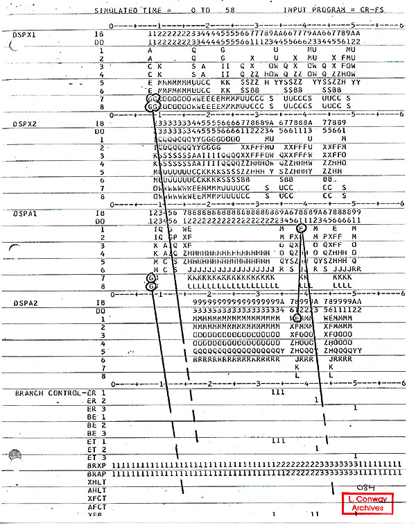
The Timing Charts: A set of timing charts are produced for each 100 cycle period of simulated time. The general form of these charts is as follows:

 

 

The time axis has markers every cycle and number indicating 10, 20, ..., 90 cycle points in the 100 cycle period. The time of the period is listed at the top of the page (ex.: SIMULATED TIME = 300 TO 399).

 

The machine facilities included in the timing charts are identified as follows:

 

DSPX1, DSPX2, DSPA1 , DSPA2: These are the dispatch registers X1, X2, Al, A2. The IB number and DO table entry are listed which correspond to the contents of the dispatch register. The eight 24-bit instruction fields are shown for each register with markers indicating which instructions of the input trace are currently present.

 

BRANCH CONTROLS: These are hardware triggers controlling the branching process. ER1, ER2, ER3, BE1, BE2, BE3, ET1, ET2. ET3 are the exit resolved, branch executed, and exit taken entries in the Exit History Table (EHT). BRXP, BRAP are the X and A pointers to the EHT. The description of the other listed controls is beyond the scope of this introductory memo.

 

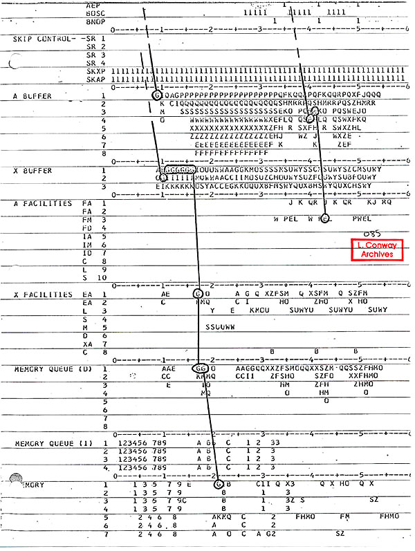
SKIP CONTROLS: Skip state triggers with SKXP, SKAP, the X and A unit pointers to the triggers.

 

 

2-9
IBM CONFIDENTIAL

 

 

A BUFFER, X BUFFER: These are the A and X unit contender stacks where ops are tested for interlocks before issuance to the functional units. This is the point where ops may be issued out of order if the appropriate interlocks are satisfied. The instruction occupancy of the buffer positions is indicated by markers.

 

A FACILITIES, X FACILITIES: These are the various functional units such as adders, multipliers, shifters, logic units, etc.

 

The instruction markers are placed in a facility position for that period of time during which the instruction actually has the facility busy for interlocking purposes. Note that an op keeps a facility busy for a number of cycles equal to the REP TIME of that facility.

 

MEMORY QUEUE (D): The data memory queue. This is the queue which holds data loads and stores after issuance from the contender stacks and before issuance to memory. This queue roughly approximates the timing effects of the BLCU with no paging activity. If appropriate interlocks are satisfied the requests may go out of order. An instruction is indicated by its marker.

 

MEMORY QUEUE (I): Instruction fetch memory queue. This queue holds the instruction fetch requests prior to issuance to memory. The markers are the IB destination number of the fetch. Four markers are placed corresponding to the four pieces of one request. When all have been issued a new set may enter.

 

MEMORY: Here we can observe the relative timing of loads, stores and instruction fetches as their markers indicate busy memory BOMS. The marker for an instruction is placed on the second of the two cycles that the op is activating the BOM--noting that the memory BOM REP TIME is one cycle.

 

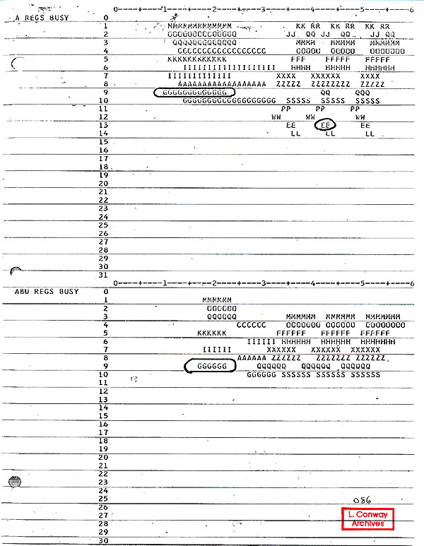
A REGS BUSY: When an OP is issued from the A contender stack to a functional unit, the A destination register of the OP is marked busy with the OP marker. This is used to interlock the issuance of other OPS in the contender stack (which use that destination register) until the result arrives at the register ( or is available for bypassing to the input of another facility).

 

 

2-10
IBM CONFIDENTIAL

 

 

ABU REGS BUSY: The A Back-Up Registers are the destination registers for A loads and X to A moves (instructions issued from the X unit contender stack). At the time of issuance the op marker is placed in the ABU REGS BUSY position corresponding to the op destination and remains till the load or move is completed.

 

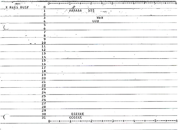
X REGS BUSY: The busy bits for the X Registers, similar to the A REGS BUSY described above.

 

 

Example of Timing Simulator Output

 

At the end of this section is a copy of the output listing for a typical run of the Timing Simulator. The parameter page is followed by 3 pages listing the input trace for the first 100 cycle period of time. Then 4 pages are listed containing the timing charts for the first 100 cycles.

 

The program being timed is a version of Crout Reduction. In this case the MPM is active for only 58 simulated machine cycles--a starting transient is followed by three passes through the inner loop of the program.

 

The interpretation of the timing charts can be somewhat complex. In this memo only a few simple illustrative examples are given which follow the paths of certain instructions of the sample program through the various sections of the machine.

 

A thorough knowledge of the MPM hardware controls and considerable practice are necessary for a complete interpretation of the timing charts. However, certain subsets of the charts maybe studied with a detailed knowledge of only that section of the MPM. For example, someone interested in compiler scheduling of instructions could focus his attention on the performance of his input programs in the A and X BUFFERS and A and X FACILITIES, observing the effects of various schedulings on the timing through these units. A knowledge of the interlocking rules of the contender stacks and of the busing and facility structure would be sufficient to get a start at this.

 

Certain simple observations may yield useful measures of MPM performance on the input program. The overall time of the run is easily determined. It is given as the upper time limit on the last set of pages listing timing charts for the run. In our example this overall run time is 58 cycles. Another measure which is often useful is the time taken to execute a program loop. If the input program is of the type

 

 

2-11
IBM CONFIDENTIAL

 

 

which repetitively executes a loop, the loop pattern will be obvious in the A and X FACILITY busy markers on the timing charts. This is because a given op has the same marker symbol each time the loop is executed (the marker is determined by the instruction address). Thus the loop time is found by measuring from marker to similar marker in the A FACILITIES for example. In our sample output we find that the MPM executes the program loop 3 times in the, FLOATING MULTIPLIER between cycle 33 and cycle 52. The pattern has not yet settled down to a repetitive one in the example, but the loop time is seen to be approximately 8 cycles.

 

Some detailed examples follow. Refer to the sample listings at the end of this section.

 

Instruction Fetching: At time = 1 an instruction fetch request to fill IB(1) has been placed on the MEMORY QUEUE (1). It is issued to MEMORY in the next cycle and (after some busing time) we observe at time = 4 that MEMORY BOMS 1, 2, 3, 4 are busy servicing this request. The fetched instruction is then bused to IB(1) (not indicated in output). At time = 8 we observe that DSPX1 and DSPA1 have been loaded from IB(1). The instructions which were fetched are seen to be A, C, E, G, which are X OPS and in DSPX1, and G which is an A OP and in DSPA1.

 

Notice that instruction fetching occurs up to time = 33. After this time the loop has been contained in the IB's and no further instruction fetching is required to run the problem.

 

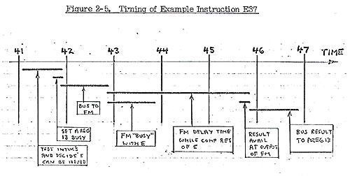
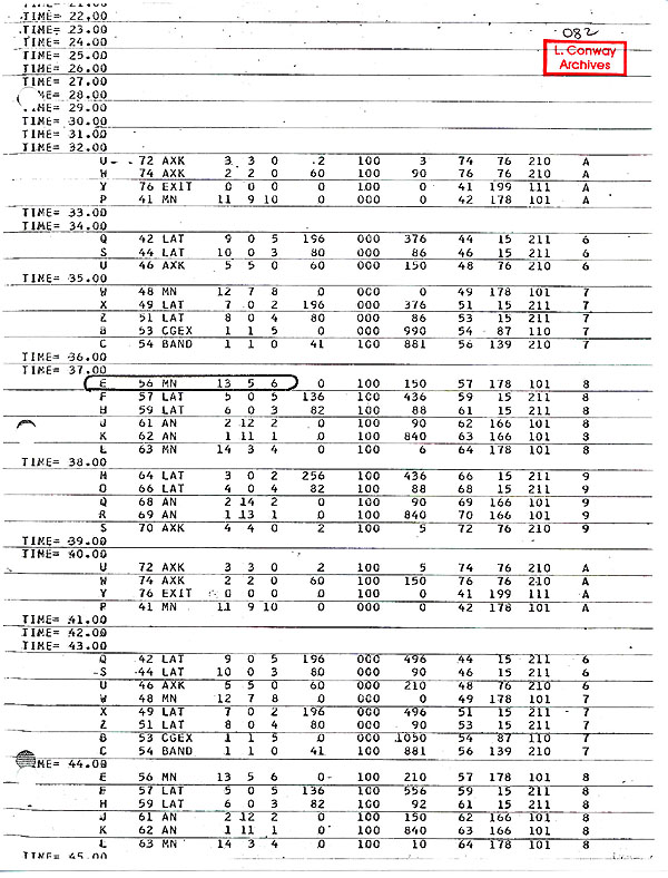
Multiply Instruction E37: At time = 37 we find the instruction MN 13, 5, 6, which is marked by an "E", in the instruction trace section of the output.

 

Let us follow the activity of this instruction through the MPM. We observe from the trace that E was fetched into IB(8). At time = 38 we notice that IB(8) >DSPA2 and we find E in DSPA2(1). At time = 38 only two positions are free in the A BUFFER so the OPS X and Y in DSPA1 move to the A BUFFER at time = 39 but E remains in the dispatchers, moving up to DSPA1(l).

 

At time = 39, the A BUFFER has two free positions so at time = 40 instruction E along with F are bused to the A BUFFER. We find E in A BUFFER (4) at a time = 40.

 

 

2-12
IBM CONFIDENTIAL

 

 

Now at time = 40 another multiply instruction, P, is present in the A BUFFER and ahead of E. This multiply, interlocking E, is issued the next cycle while E remains present at time = 41 in A BUFFER (3). At this time there are no ops ahead of it in the buffer which interlock it so it is issued for execution and is not present in A BUFFER at time 42. Notice that A REG BUSY (13) goes on with the marker E at time = 42 to interlock any OPS following E which -use A REG (13) as a source or destination.

 

The multiplier FM under A FACILITIES is found busy with E at cycle time = 43 (one cycle of busing required from A BUFFER to A FACILITIES). Then at time = 44 the A REG BUSY (13) is no longer marked by E indicating that the result of E will be available (for bypassing) at the output of the multiplier at cycle time = 46. Note that the delay time of the FM is 3 cycles, the multiply E taking cycles 43, 44, 45, with the result actually back at register 13 at cycle 47. But the multiplier is only "busy" with E for one cycle (the REP TIME of FM) so the multiplier could handle a new op every cycle. The timing of the busing and multiplication are illustrated in Fig. 2-5, for the specific example instruction E37.

 

 

 

 

2-13
IBM CONFIDENTIAL

 

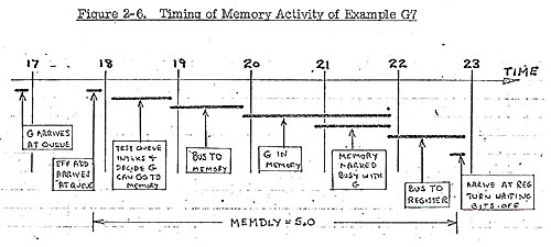
Arithmetic Load Instruction G7: At time = 7 we find the instruction LAT 9, 0, 31, 136 which is marked by a "G", in the instruction trace section of the output. We observe from the trace that G was fetched into IB(1). It is both an AOP and an XOP and will be dispatched to both units.

 

At time = 8, we observe from the timing charts that IB(1) > DSPX1, IBM > DSPA1. At that time G is present in DSPX1(7), DSPX1(8), and in DSPA1(7), DSPA1(8). G is a long OP and takes two of the 24-bit positions in the dispatchers.

 

Let us follow the A unit activity of G first. We note that at time = 8 G is the first AOP to enter the dispatchers and thus it is bused to the A BUFFER the next cycle. At time = 9 we find G in A BUFFER (1). This part of G is a "replace" operation and is issued the next cycle, causing A REG BUSY (9) (the destination of the load) to be marked busy with a G at time = 10. This sets the "front" register busy waiting for the "back-up" register to be loaded by the X-unit.

 

Now let us follow the X unit activity of G. Since three other X OPS precede G in DSPX1 at time = 8, and at most 3 ops may be dispatched to the X BUFFER per cycle, G remains in DSPX1 at time = 9. At time = 10 it is bused to X BUFFER (2), for it is the next op to be dispatched to the X BUFFER and both A and C leave the X BUFFER at time = 10 allowing G to enter.

 

We now find that G remains in the X BUFFER through time = 16. This is because it uses X REG (31) as an index and X REG (31) is busy through time = 15 waiting for a load to arrive.

 

At time = 16 G finally satisfies the contender stack interlocks and at time = 17 its execution is initiated by (i) starting effective address computation in X FACILITY EA1, (ii) placing an entry in the MEMORY QUEUE (D), (iii) marking the ABU REG BUSY (9) with G. The queue entry waits on the queue another cycle for the effective address to arrive, and then is issued to memory. We note that at time = 21, MEMORY (1) is marked busy with G, and at time = 23 the busy. bits on ABU (9) and A(9) are turned off indicating that the load has arrived at ABU (9) and then moved immediately to the waiting A(9).

 

The detailed timing of this memory activity is illustrated in Fig. 2-6.

 

2-14

 

 

2-15 (MPM timing simulator input for CR-FS):

 

2-16

 

2-17

 

2-18

 

2-19 (MPM timing simulator output for input CR-FS):

 

2-20

 

2-21

 

2-22

 

 

3-1
IBM CONFIDENTIAL

 

 

CURRENT JOB RUNNING PROCEDURES

 

This section describes the procedures to be followed in order to use the timing simulation program. These procedures are to be completely revised and expanded in the near future so that the programs may be stored on disk at the MOD 75 comp lab and users may submit runs directly at the comp lab (see Section 5).

 

To use the timing simulator at the present time:

 

(i) Write the assembly code input program for the Unroller (Section 1).

(ii) Prepare the machine parameter card required for the Timer input deck (Section 2).

(iii) Submit these items to L. Conway, Room 203, Extension 252.

 

 

4-1
IBM CONFIDENTIAL

 

 

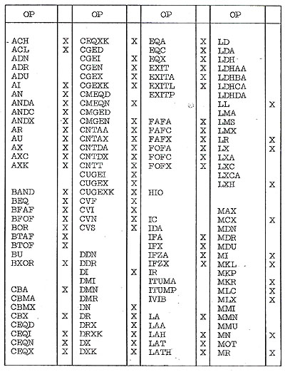
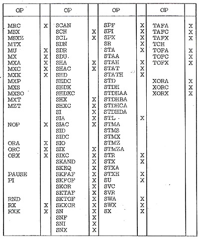
TABLE OF IMPLEMENTED INSTRUCTIONS

 

The table on the following pages lists the ACS-1 instruction set op codes and indicates (with an X) if a given op is implemented in the Timing Simulator.

 

 

4-2

 

 

4-3

 

 

5-1
IBM CONFIDENTIAL

 

 

PLANNED MODIFICATIONS

 

Certain modifications to the simulation programs are now being made or are planned for the near future. These are briefly described below to assist users in their planning. Updates to this memo will. be issued as these changes are included in the programs.

 

Unroller Changes

 

The control specification facilities will be extended.

 

 

Timing Simulator Changes

 

(ii) Additional OPS will be implemented.
(ii) New output features and options will be added.

 

 

Job Running Procedure Changes

 

Currently jobs must be submitted to L. Conway who will handle the processing of the jobs. Two separate programs must be run consecutively to process one timing simulation. This results in a rather long overall turn-around time. To improve on this, the two programs will be merged, with the trace temporarily stored in core or on disk and automatically passed between them.

 

Also, the program will be placed on disk at the MOD 75 comp lab. The running of jobs will then be handled directly by the user, who will submit the assembly code input deck, parameter card, and appropriate JCL cards to call for the timing simulator.

 

These changes will greatly reduce overall turn-around time and allow a much greater number of users to be served than is now possible.

 

lynnconway.com > ACS Archive front-matter > IBM-ACS MPM Timing Simulator